The correlation coefficient is a fundamental statistical measure that quantifies the strength and direction of a linear relationship between two variables. When two sets of data are strongly linked together, they are said to have a high correlation. This value provides insight into how well the relationship between variables can be represented by a straight line, indicating whether the association is positive or negative.
What is Correlation?
Correlation, also known as statistical association, describes the extent to which the value of one variable can predict the value of another. For independent variables, the correlation is zero, signifying no discernible relationship.
Types of Correlation
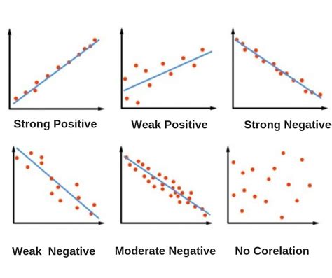
- Positive Correlation: When one variable increases, the second variable usually also increases, and vice versa. On a scatter plot, the data points typically angle upwards from left to right.
- Negative Correlation: When one variable increases, the second variable usually decreases, and vice versa. On a scatter plot, the data points typically angle downwards from left to right.
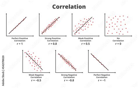
- Perfect Correlation: In a perfect correlation, knowing the value of one variable allows for the exact calculation of the second variable's value. A perfect positive correlation is represented by
r = 1, while a perfect negative correlation isr = -1.
The correlation coefficient is a unit-free value that ranges between -1 and 1. The absolute value of the correlation coefficient indicates the strength of the relationship. A larger absolute value signifies a stronger relationship. For instance, |-0.75| = 0.75 indicates a stronger relationship than 0.65.
Pearson's Correlation Coefficient: The Most Common Measure
Pearson's correlation coefficient, often denoted as Pearson's r, is a widely used statistic that measures the linear association between two continuous variables. It is a parametric test, meaning it assumes certain characteristics about the data, such as a bivariate normal distribution.
How to Calculate Pearson's Correlation Coefficient
The calculation of Pearson's r involves comparing the deviation of each data point from the mean of its respective variable. The formula for the sample Pearson correlation coefficient is:
$r = \frac{\sum(xi - \bar{x})(yi - \bar{y})}{\sqrt{\sum(xi - \bar{x})^2\sum(yi - \bar{y})^2}}$
This formula can also be expressed using covariance and standard deviations:
$r = \frac{Cov(X,Y)}{\sigmaX \sigmaY}$
Where:
- $Cov(X,Y)$ is the covariance between variables X and Y.
- $\sigma_X$ is the standard deviation of variable X.
- $\sigma_Y$ is the standard deviation of variable Y.
The calculation can be done in a single pass through the data, and software like Excel (using the CORREL() function) or LibreOffice Calc can easily compute it.
Assumptions for Pearson's Correlation
For Pearson's r to be a reliable measure, several assumptions should ideally be met:
- Continuous Variables: Both variables should be continuous (measured on an interval or ratio scale).
- Linearity: There should be a linear relationship between the two variables. A scatter plot is crucial for visually assessing this.
- Outliers: The sample correlation value is sensitive to outliers. Extreme values can significantly skew the coefficient. Pairwise analysis and examination of linear regression residuals are important for detecting outliers.
- Normality: Ideally, the data should follow a bivariate normal distribution. However, in practice, checking the normality of linear regression residuals is often sufficient.
- Homoscedasticity: The variance of the residuals should be constant across all levels of the independent variable.
Correlation Effect Size
The correlation value itself serves as a measure of the correlation effect size. While interpreting the strength of a correlation can be subjective and context-dependent, general guidelines exist. Following Cohen's (1988) guidelines:
| Correlation Value ( | r | ) | Level |
|---|---|---|---|
| < 0.1 | Very small | ||
| 0.1 ⤠| r | < 0.3 | Small |
| 0.3 ⤠| r | < 0.5 | Medium |
| ⥠0.5 | Large |
It is important to remember that these are rules of thumb, and the "meaningful" size of a correlation can vary significantly across different disciplines and research contexts.
Beyond Linearity: Spearman's Rank Correlation Coefficient
When the assumptions for Pearson's correlation are not met, particularly concerning linearity or data distribution, Spearman's rank correlation coefficient offers a robust alternative. It is a non-parametric statistic that measures the monotonic association between two variables. A monotonic association means that as one variable increases, the other variable consistently increases or consistently decreases, but not necessarily at a constant rate.
When to Use Spearman's Rank Correlation
Spearman's rank correlation is suitable for:
- Ordinal Discrete Variables: When variables are ranked or ordered.
- Non-linear Data: When the relationship between variables is monotonic but not strictly linear.
- Data Distribution Issues: When the data distribution is not bivariate normal.
- Presence of Outliers: Spearman's is less sensitive to outliers than Pearson's r.
- Non-Homoscedasticity: When the variance of residuals is not constant.
How to Calculate Spearman's Rank Correlation
The calculation involves ranking the data for each variable separately and then computing the Pearson correlation coefficient on these ranked data. The smallest value is assigned a rank of 1, the second smallest a rank of 2, and so on.
Handling Ties: When data contains repeated values, each tied value receives the average of the ranks they would have occupied. For example, if two values share the 4th and 5th ranks, both would be assigned a rank of (4+5)/2 = 4.5.
The symbol for Spearman's rank correlation coefficient is $\rho$ (rho) for the population and $r_s$ for the sample. If the correlation coefficient is 1, all rankings for each variable match perfectly for every data pair. A coefficient of -1 indicates that the rankings for one variable are the exact opposite of the rankings for the other variable.
Covariance: The Precursor to Correlation
Before diving deeper into correlation, understanding covariance is essential. Covariance measures the relationship between two variables, indicating whether they tend to move in the same or opposite directions.
Understanding Covariance
- Range: The covariance range is unlimited, extending from negative infinity to positive infinity.
- Zero Covariance: For independent variables, the covariance is zero.
- Positive Covariance: Indicates that changes in the variables occur in the same direction. When one variable increases, the second variable usually also increases, and vice versa.
- Negative Covariance: Indicates that changes occur in opposite directions. When one variable increases, the second variable usually decreases, and vice versa.
How to Calculate Covariance
The formula for covariance is:
$Cov(X,Y) = E[(X - E[X])(Y - E[Y])]$
Or, more practically for sample data:
$S{XY} = \frac{\sum(xi - \bar{x})(y_i - \bar{y})}{n-1}$
Where $S_{XY}$ is the sample covariance between X and Y, $\bar{x}$ and $\bar{y}$ are the sample means, and $n$ is the number of data points.
The Nuance of Correlation: "Correlation Is Not Causation"
A crucial principle in statistical analysis is that correlation does not imply causation. While a strong correlation might suggest a relationship, it does not inherently mean that one variable causes the other. There can be numerous reasons for an observed correlation:
- Third Variable: A hidden, third variable (Z) might be influencing both variables (X and Y), creating an apparent relationship. For example, poor suburbs are more likely to have high pollution. This doesn't mean poor people cause pollution; rather, factors like factories with low-paying jobs and significant pollution might be common links.
- Random Chance: Especially with small sample sizes, a strong correlation might arise purely by chance.
- Reverse Causation: The direction of causality might be reversed. For instance, in a survey, a strong positive correlation between studying an external course and sick days might lead one to question if studying makes people sick, or if sick people are more likely to study.
Correlation vs Causation (Statistics)
The Ice Cream Example: When Lines Don't Tell the Whole Story
Consider the example of an ice cream shop tracking sales against temperature. Initially, warmer weather correlates with higher sales (e.g., r = 0.9575). This indicates a strong positive linear relationship. However, during a heatwave, extreme temperatures might deter customers, causing sales to drop. If one were to calculate the correlation coefficient for this entire dataset, the value might approach zero (r = 0), indicating "no correlation."
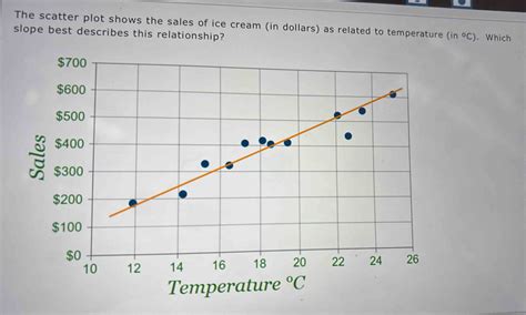
This scenario highlights a limitation of correlation coefficients, particularly Pearson's r, which assumes linearity. The data might follow a distinct curve, reaching a peak sales point around a certain temperature (e.g., 25°C), but the correlation calculation is not "smart" enough to recognize this non-linear pattern. In such cases, a visual inspection of a scatter plot or the use of Spearman's rank correlation might reveal the underlying monotonic trend.
Correlation Coefficient Formulas and Calculations
The correlation coefficient formula is used to determine how strongly two datasets are related.
Pearson's Product Moment Correlation (PPMC)
This is the most common type of correlation. It quantifies the strength of the linear relationship between two continuous variables.
Manual Calculation Steps (Simplified Example):
Let's consider a simplified dataset for Ice Cream Sales (X) and Temperature (Y):
| Sales (X) | Temperature (Y) |
|---|---|
| 43 | 99 |
| 99 | 75 |
| 45 | 70 |
| 70 | 80 |
| 75 | 85 |
Calculate the Mean:
- Mean of Sales ($\bar{x}$) = (43 + 99 + 45 + 70 + 75) / 5 = 66
- Mean of Temperature ($\bar{y}$) = (99 + 75 + 70 + 80 + 85) / 5 = 81.8
Calculate Deviations from the Mean:
- For Sales: (43-66), (99-66), (45-66), (70-66), (75-66) = -23, 33, -21, 4, 9
- For Temperature: (99-81.8), (75-81.8), (70-81.8), (80-81.8), (85-81.8) = 17.2, -6.8, -11.8, -1.8, 3.2
Calculate the Product of Deviations:
- (-23 * 17.2), (33 * -6.8), (-21 * -11.8), (4 * -1.8), (9 * 3.2) = -395.6, -224.4, 247.8, -7.2, 28.8
Sum the Products of Deviations (Numerator):
- -395.6 - 224.4 + 247.8 - 7.2 + 28.8 = -350.6
Calculate the Sum of Squared Deviations for X:
- $(-23)^2 + (33)^2 + (-21)^2 + (4)^2 + (9)^2 = 529 + 1089 + 441 + 16 + 81 = 2156$
Calculate the Sum of Squared Deviations for Y:
- $(17.2)^2 + (-6.8)^2 + (-11.8)^2 + (-1.8)^2 + (3.2)^2 = 295.84 + 46.24 + 139.24 + 3.24 + 10.24 = 494.8$
Calculate the Denominator:
- $\sqrt{(2156) * (494.8)} = \sqrt{1066716.8} \approx 1032.82$
Calculate the Correlation Coefficient (r):
- $r = \frac{-350.6}{1032.82} \approx -0.339$
This example, while simplified, demonstrates the manual process. The negative correlation suggests that in this specific (and likely contrived) dataset, higher temperatures are associated with lower sales, which is counterintuitive for an ice cream shop and highlights the importance of realistic data and context.
Using Software for Calculation
You will rarely need to calculate these coefficients by hand. Various software tools can perform these calculations efficiently:
- Excel/LibreOffice Calc: The
CORREL()function.- Enter your data into two columns.
- Select a cell for the result.
- Type
=CORREL(array1, array2), wherearray1andarray2are the ranges of your data columns.
- SPSS: Navigate to "Analyze" > "Correlate" > "Bivariate." Select variables, choose "Pearson," and specify the test type (one-tailed or two-tailed).
- Minitab: Go to "Stat" > "Basic Statistics" > "Correlation." Select the variables, and optionally check the "P-Value" box.

Statistical Significance of Correlation
A calculated correlation coefficient tells us about the relationship in our sample data. However, to generalize this finding to the broader population, we need to assess its statistical significance. This is typically done using a p-value.
Hypothesis Testing in Correlation
- Null Hypothesis ($H_0$): The observed correlation in the sample is due to random chance, meaning there is no actual linear relationship between the variables in the population ($\rho = 0$).
- Alternative Hypothesis ($H_1$): The observed correlation is real and reflects a genuine relationship in the population ($\rho \neq 0$).
A low p-value (typically less than 0.05) suggests that the observed correlation is unlikely to have occurred by chance, leading us to reject the null hypothesis and conclude that a statistically significant relationship exists.
Correlation Tests
- T-test: When the null hypothesis is $\rho = 0$ and the variables have a bivariate normal distribution or the sample size is large, a t-test can be used.
- Fisher Transformation: For situations where the null hypothesis is not $\rho = 0$, or when dealing with smaller sample sizes where the distribution might not be symmetrical, the Fisher transformation can be applied to the correlation coefficient to make its distribution more symmetrical, allowing for the use of z-tests.
Other Types of Correlation Coefficients
While Pearson's r and Spearman's rho are the most common, several other correlation coefficients exist, each suited for different types of data and relationships:
- Kendall's Tau: Another non-parametric measure for monotonic association, particularly useful for smaller sample sizes or data with many ties.
- Concordance Correlation Coefficient (CCC): Measures the agreement between two sets of measurements, assessing how well data aligns with a "gold standard."
- Intraclass Correlation (ICC): Evaluates the consistency of ratings or measurements within groups or clusters, often used for inter-rater reliability.
- Matthews Correlation Coefficient (MCC): A balanced measure for binary classification problems, considering true positives, true negatives, false positives, and false negatives.
- Moran's I: Quantifies spatial autocorrelation, measuring the similarity between objects in close proximity.
- Phi Coefficient: Measures the association between two binary variables.
- Point Biserial Correlation ($r_{pb}$): A special case of Pearson's r used when one variable is continuous and the other is dichotomous.
- Polychoric Correlation: Measures the association between two ordinal variables.
- Tetrachoric Correlation: Measures rater agreement for binary data.
- Cramer's V: Used for measuring correlation in contingency tables with more than two rows and columns.
The choice of correlation coefficient depends heavily on the nature of the variables being analyzed and the type of relationship being investigated. Always consider visualizing your data with a scatter plot before calculating any correlation coefficient to ensure the chosen method is appropriate.
tags: #how #to #calculate #corelation